Do you have a spreadsheet with too many columns, and a small amount of information in each? Maybe you have the address split up in 6 columns: house number, street name, rd/ave/dr/st etc., city, state, zip. Or possibly your spreadsheet contains a lot of auto information in separate columns that you would like to combine (auto, make, year, color, etc.). You may want to consider editing your spreadsheet before importing it into Blitz Sales Follow-Up Software to best utilize the 20 available custom fields or to properly match up with the basic contact information. Making a decision on how to organize your information before entering it into the system can save you a lot of time and headache later on, and will make lead tracking a much simpler process for you and your staff.
How to combine two or more columns in Excel:
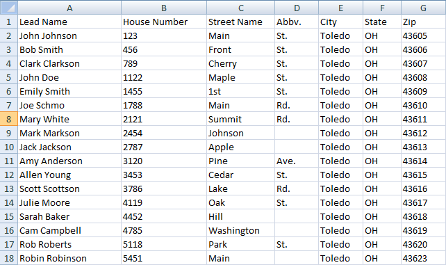
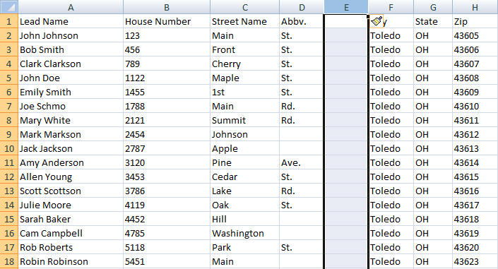
- Decide which columns you would like to combine. Below is an example of a spreadsheet with house number, street name, and abbv. in three separate columns. In Blitz, you would want to put these all in the “Address 1” field, so it would be best to combine these into one column.
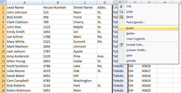
- Create a new column for the combined data to be added to. To add a new column, right click on a column to the right and select “Insert.”
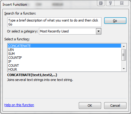
- In the top cell of the new blank column created in step 2, add a concatenate function. The easiest way to do this is to click the fx button to the left of the wide text box above your spreadsheet that displays the current cell data.
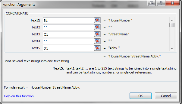
After clicking the fx button, an assistant dialogue will pop up and help you create the function.Type concatenate at the top to find the function. Select it and click OK.The next box will ask you which cells you would like to combine. Since you are adding the function in the top cell, you will want to type the top cells of each column you are combining with a space in between each. In the example below, I am combining columns B, C, and D, so I typed B1, C1, and D1 in separate “Text boxes” within the dialogue. In between each, I typed a space to make sure there is a space between each value (the quotation marks are added automatically). At the bottom of the dialogue it will tell you what the formula result looks like. Click OK when complete.
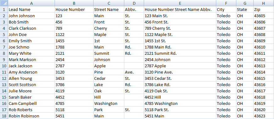
- To apply this function to the rest of the rows in your spreadsheet, click the small square at the bottom right of the cell containing the formula. Drag your mouse down until you reach the bottom of your spreadsheet.
End result:


 The next box will ask you which cells you would like to combine. Since you are adding the function in the top cell, you will want to type the top cells of each column you are combining with a space in between each. In the example below, I am combining columns B, C, and D, so I typed B1, C1, and D1 in separate “Text boxes” within the dialogue. In between each, I typed a space to make sure there is a space between each value (the quotation marks are added automatically). At the bottom of the dialogue it will tell you what the formula result looks like. Click OK when complete.