The larger your database grows, the tougher it is to keep the data clean. Fortunately, Excel provides a simple way to either highlight or remove duplicate data. Below are two methods:
Highlight the duplicate data
If you would like to further analyze the data before deleting or editing it, use this option. Click here for instructions on exporting from Blitz.
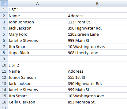
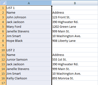
- If you would like to compare two lists, copy one list and paste it underneath another list. Make sure the columns match up, as below:
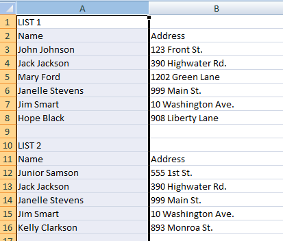
- Highlight the column you would like to base the duplicate check on. In this example, we are searching based on name, but you could also search by phone number, email, etc.
- Under the Home tab, select Conditional Formatting > Highlight Cell Rules > Duplicate Values
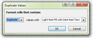
- Choose to format cells that contain duplicate values with (any style you choose). Click OK.
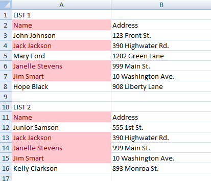
- The duplicate cells are now highlighted:
Remove the duplicate data
Go this route if you would like to get rid of duplicate rows. Click here for instructions on exporting from Blitz.
- If you would like to compare two lists, copy one list and paste it underneath another list. Make sure the columns match up, as below. Highlight the column you would like to base the duplicate check on.
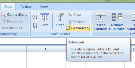
- In the Data tab, select Advanced Filter:
- Choose “Filter the list, in-place” for the action, and check “Unique records only.” Click OK.
- The duplicates are now removed:

